AC Circuits

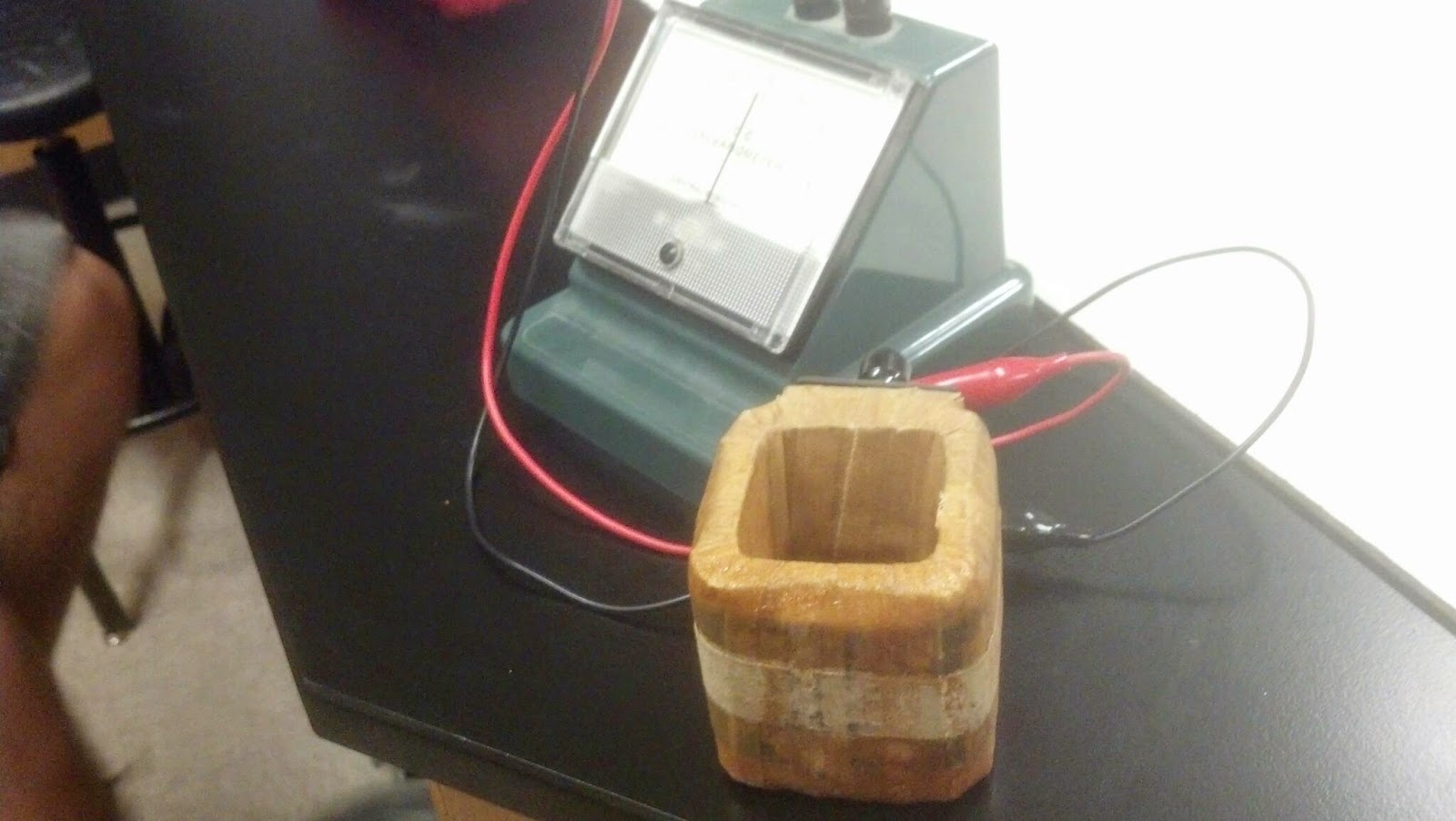
     I am not exactly sure what was in this box, but this is the setup for a demonstration Professor Mason performed in class on Monday. The purpose of the demonstration was to show a particular difference between DC voltage and AC voltage. Initially, one half of the box was lit up through a 3 volt DC power source and the other half through a 3 volt AC source. The side lit up by the DC source was much brighter. The sides of the box were not equally as bright until the AC source was turned up to around 4.6 V AC, which is roughly 3 volts RMS. 

 

     In lab, we conducted an experiment in which we calculated a theoretical capacitive reactance and then used current and voltage sensors to construct graphs using LoggerPro that would be used to determine RMS voltages and currents. These voltages and currents would be used to acquire another value of capacitive reactance that we would compare to our theoretical value. We did this for two different capacitors and then found that doubling the frequency greatly reduced our percentage error. We attempted a similar process with an inductor, but found that our results we not nearly as accurate as they were with the capacitor. Also, we simply ran out of time to complete the inductor experiment in its entirety.  

 

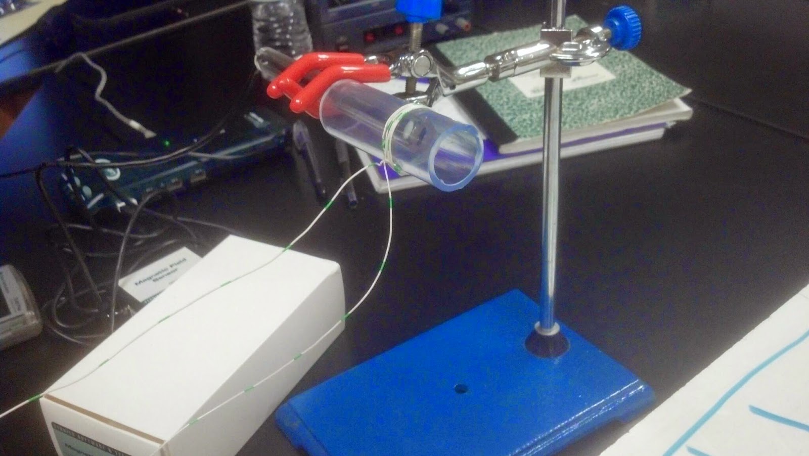
     This is a sample of the graphs we obtained through use of the voltage and current sensors hooked up into our RC circuit. In order to obtain RMS values for voltage and current, we simply took the maximum value and divided it by the square root of two. We then divided the RMS voltage by the RMS current, which gave us a value of reactance. 

Induction

     In addition to answering a number of questions on the ActivPhysics website on Wednesday, we conducted in an experiment in which we were to determine the inductance of the coil in the above picture. We calculated the inductance by using the dimensions of the coil and also by using the oscilloscope to estimate the half time of exponential decay. 

     The answer in the box is the actual inductance that Professor Mason measured while the larger value is the value we came up with using the half time of exponential decay. As one can see, our calculation was not very accurate. 

 

     This is the calculation of the coil's inductance using the dimensions of the coil. It is much closer to the true value than the previous calculation. 

Electromagnetic Induction

 

     On Monday, we measured the magnetic field of a current carrying loop with multiple loops. This is a picture of our setup. 

 

     This is a table of the values we measured during the experiment. As one can see, the values of the strength of the magnetic field were not very reliable because of the orientation of the sensor. The values to the very right are values measured by Professor Mason. 

 

     Using Professor Mason's values, we determined a constant for the value of B/NI and used that constant to calculate the length of the coil of wire. 

 

     We were also given a coil of wire on Monday and connected it to a galvanometer  in order to experiment with electromagnetic induction. We used a bar magnet in this experiment and found that factors such as the number of coils and the velocity in which we moved the magnet in and out of the coil contributed to the amount of current we measured.

 

     This is a demonstration performed by Professor Mason in which a current was given to a driver coil and a current was induced inside the smaller coil. We observed that the voltage induced in the smaller coil was smaller and 180 degrees out of phase with the voltage that was supplied to the driver coil.

Biot Savart Law

     The first thing we did in class on Wednesday was learn how to derive an expression for a magnetic field at a point a distance from an infinitely long wire. We then used that technique to come up with an expression for the magnetic field at a point in the center of a square made from four current carrying conductors. However, I think I may have made  an error in my calculation. 

 

     We also came up with an expression for the magnetic field at a point in the center of a current carrying loop. This expression was much simpler to come up with. 

 

     This is a picture of the setup of an experiment we conducted in which we were to approximate the horizontal component of the earth's magnetic field in the Physics 4B room.  We applied a small amount of current to the coil, recorded the angular displacement of the compass needle, and calculated the magnetic field in the center of the coil. We then made a graph of the magnetic field vs. angular displacement. The slope of this graph would be our approximation of the component of the earth's magnetic field which we were to determine.

     These are the calculations for the magnetic field at the center of the coil. We used these values as the four data points in our graph.

 

     This is the graph we ultimately came up with after conducting the previously described experiment. According to the graph, the component of the earth's magnetic field which we sought was on the order of 2.8*10^-5. Was this correct? I haven't the slightest idea, but it was very similar to values that other groups came up with. 

     The very last thing we did in lab was calculate the strength of the magnetic field at the center of a solenoid and compare it to the value that Professor Wolfe measured. The values were surprisingly close considering the "solenoid" used in the demonstration. 

 

DC Motors and Magnetic Fields from a Current Carrying Wire

   Because of a terrible internet connection at Mt. SAC, this is my THIRD time publishing this same post. Please excuse the fact that I lost my patience, and it is not as detailed as it originally was.    

     We were given a simple DC motor in order to observe how it worked before we were to construct our own.

 

 

     This is the simple DC motor that we constructed in lab. It worked very well actually. 

  

     In this demonstration, there was a current running through the rod, and we were to predict which direction the needles of the compasses would point. Of course, there is a right hand rule for such a prediction.

      

 

     This is an example of a prediction for the previously described demonstration. 

 

     This was a demonstration to show that magnetic fields caused by a current carrying wire do superimpose. 

Magnetic Fields and Forces

     The first thing we did in lab on Wednesday was observe the behavior of a compass when it was placed in proximity of a bar magnet. The arrows drawn on the whiteboard represent the direction of the red portion of the compass needle as it was moved in a circle around the magnet. The purpose of doing this was to get an idea of what a magnetic field looks like. 

     This is a more accurate depiction of what a magnetic field actually looks like in two dimensions. Iron shavings were placed around the bar magnetic, and they arranged themselves in the pattern shown. The field lines are nearly linear as they leave the north pole of the magnet and curve around the length of the magnet before straightening out again as they reenter the south pole. 

     This picture shows three different enclosed surfaces drawn around certain points of the magnetic field. The surface drawn to the left and the surface surrounding both poles have a net flux of zero because the same amount of field lines enter them as do exit them. The surface containing only the south pole does have a net flux of 10. However, it is important to note that a monopole magnet does not exist in nature. 

 

     These are the calculations performed to find the strength of the magnetic field in an experiment that I should have taken a picture of.  Essentially, the experiment consisted of a magnetic force created from a current running through a wire and a magnet and a hollow copper rod that rolled off a platform upon experiencing the force. All of the measurements we needed are written down toward the lower right hand corner of the white board. The final equation we derived to calculate the strength of the magnetic field is shown in green, and the answer we came up with was roughly .0207T, which seems reasonable.

     There was also another demonstration which I neglected to take a picture of. This demonstration consisted simply of a magnet and a wire with a current running through it, and we were supposed to predict which direction the magnetic force would cause the wire to move in.

 

Amplifier Circuits

     This is the schematic for a simple transistor audio amplifier circuit which we were to construct during our lab on Monday.

      This is a picture of the actual circuit which was constructed from the schematic at the beginning of this post.

     This is what we measured from the previously posted circuit using an oscilloscope. The sinusoidal function is the input from the function generator, and the wave form that is clipped on the top is the actual output of the transistor circuit.

     We also constructed another amplifier circuit in lab that used an IC and was much simpler than the previous circuit. We hooked up a phone to provide an audio signal as an input and used a speaker as the output device. The circuit worked, and the signal was indeed amplified.

     

Working With Oscilloscopes

 

     Before we began working with the oscilloscope on Wednesday, we experimented a bit with a function generator that was  hooked up to a small speaker. We initially had the function generator set to provide a sinusoidal output at 96 Hz which caused the speaker to emit a low buzz. We then noted that a square wave created a louder buzz and that a triangle wave created a lower buzz. We also noticed that changing the frequency altered the pitch and that increasing the amplitude created a louder, more intense sound.

 

     The first thing we did with this rather ancient oscilloscope was connect a battery in series with a tap key in order to measure the voltage of the battery. We had the VOLTS/DIV knob set to 1 Volt per division and observed that the voltage of the battery was roughly 1.5 Volts as it should be. 

 

     This is a picture of what the oscilloscope displayed when we connected it to a DC power supply set at 4.5 Volts. This picture shows that the quality of the power supply is not all that great because of all the noise it produces. We were  supposed to determine the amplitude of the noise, but this task turned out to be next to impossible with this particular oscilloscope.

 

     Another task that proved to be difficult to carry out with this oscilloscope was to create lissajous figures when the oscilloscope was hooked up to both an AC transformer and the function generator. The picture above and the two below are examples of such figures when the function generator is set provide frequencies of 60 Hz and multiples of 60 Hz. 

 

     This is a picture of the diagram we constructed from our experiment with the "Mystery Box" we were provided in lab. There were a total of ten possible combinations that we could measure the output from using the oscilloscope. We could not determine exactly what was in the box, but it appears that there were some batteries of some kind and also perhaps a transistor that was producing a square wave. 

RC Circuits

     This is the setup for the lab we conducted on Monday in which we were to create graphs of  a capacitor's charging and discharging times using LoggerPro.

 

     This is the graph of electric potential vs. time that was created during the experiment. It shows that a capacitor charges and discharges not linearly, but asymptotically. It also shows that the charging and discharging levels off at a certain point and that the capacitor will never really reach its maximum charge.

      After the experiment was completed, we compared the value of "c" from the fit equation of the discharging graph to a value we calculated from the values of the components used in the experiment. Because the numbers are so small, there is actually quite a large percentage error of about 32% if our calculated value of .01027 is taken to be the "true" value.

Capacitance

 

     On Monday, we conducted an experiment in which we turned a book into a capacitor. It is difficult to see from the picture, but there are two sheets of aluminum foil of equal area inserted into the book with pages in between them. 

 

     This is a chart of the capacitance we measured using our capacitor. For the first part, we increased the distance between the plates with the initial distance being the thickness of 10 pages. For the second part, we halved the area of the plates by simply folding the foil in half. We also attempted to calculate the true value of "k" for aluminum foil using some of our data. We were off by about a factor of three.  

 

     The above picture is a graph of capacitance vs. distance. The graph shows that capacitance is inversely proportional to the distance between the plates just as we expected it to be. 

DC Circuits

      On Wednesday, we were given a series-parallel circuit and were asked to compute the equivalent resistance of the entire circuit. We broke it down into parts in order to make that computation, and those calculations can be seen in the picture above. Then, we made the circuit by twisting resistors together, measured the total resistance, and compared it to our calculated value. Those values can be seen in the lower right hand corner of the whiteboard.

 

      The two pictures above are pictures of an exercise we also completed on Wednesday. We constructed the circuits from the schematics seen in the picture and analyzed voltage and current in both series and parallel circuits. We found that the sum of the potentials across the resistors in a series circuit equals the input voltage, and that the current is the same in all components in a series circuit. We found that the opposite was true for parallel circuits. Specifically, the sum of the currents in a parallel circuit equals the input current, and the potential is the same across all resistors in a parallel circuit.

 

     We were given another circuit and were asked to compute the three unknown currents using Kirchhoff's laws. We were then to build the circuit on a breadboard, and actually measure the currents and compare them to our measured values. However, this is still a work in progress, and a picture of the circuit can be seen below. 

 

     Our calculated values for the currents I_1, I_2, and I_3 were 1.14 amps, .999 amps, and .138 amps respectively. Upon actually breaking the circuit at the necessary points in order to measure these currents, I found that I_1, I_2, and I_3, were 1.12 amps, .99 amps, and .11 amps respectively.  

Electric potential

     The above picture shows the data collected and the graph constructed from that data for the experiment we performed on Monday. The setup of the experiment involved a DC power supply which was set to 15 volts, a multimeter, and a sheet of conductive paper pinned to a piece of particle board. The positive end of the power supply was connected to a silver painted line on the paper, and the negative end was connected to a circular painted point on the paper. We began testing the potential at the circular point and moved the positive lead of the multimeter away from the circular point in 1cm increments until we reached the silver painted line. We recorded the potential for each of these distances in excel and constructed a graph of Potential vs. Distance, which can be seen in the picture.

More Power

     We had a lovely fiesta this past Wednesday! Instead of taking a typical quiz, we were given the materials shown in the above picture and asked to construct a circuit which lit the light bulbs as dimly as possible. In order to do this, we simply connected the two batteries in parallel and hooked them up to the two light bulbs which were connected in series. 

 

     There was also an experiment performed on Wednesday which involved a resistive coil that would heat a known mass of water when voltage was applied to it. We were given the mass of the water, the dimensions of the coil, and the applied voltage. Our goal was to determine the change in temperature of the water with our given information after a period of ten minutes had elapsed. We first determined the resistance of the coil and the current flowing through it. Because other groups had used a different value of resistivity and calculated a different current, we used these two values to come up with an uncertainty for the current. We then determined the power, the energy put into the water, and finally the change in temperature with uncertainty. The actual change in temperature was 2.5 degrees Celsius, but we calculated a change of 2 + or - .49 degrees Celsius. We went through the same process with an initial voltage of 9 volts instead of 4.5 volts. Those calculations are seen in the upper portion of the whiteboard. Doubling the voltage did not double the change in temperature. My intuition told me it would not because doubling the voltage, doubles the current, which increases the power by a factor of four.

      These are some hotdogs with 120 volts passing through them. The longer, thinner one cooked more quickly because it had more resistance than the shorter one with a greater cross sectional area. Some LEDs were placed into the hot dog to show that the further the leads of the LED were placed from each other, the greater the electric potential would be between the two leads. This was proven by observing that the LED with its leads positioned furthest apart burned out almost immediately.